Statics. Translational and rotational equilibrium of a rigid body. Free-Body Diagram. Polygon method of vector addition.
In engineering it is often desired to know the forces or stresses existing in various parts of a structure or machine. One might wish to know the stresses in the various members of a bridge truss, for example. These questions are the domain of the subjects of statics and dynamics.
Def. Statics. The branch of mechanics dealing with bodies at rest and with the interactions of forces in equilibrium.
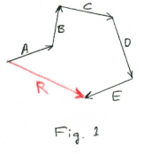
Polygon method of vector addition. This method for vector addition consists of starting at any convenient point and drawing the vectors head-to-tail as shown in Fig. 1. Here R represents the sum of vectors A, B, C, D, E.
Theorem 1. The sum of n vectors A + B + C + ..... + P + Q is the same regardless of the order in which they are summed.
Example. A + B + C = C + B + A
Def. Translational equilibrium of a rigid body. A rigid body is in translational equilibrium if it is at rest or is moving at constant speed in a straight line.
Def. Rotational equilibrium of a rigid body. A rigid body is in rotational equilibrium if it is not rotating, or if it is rotating at a constant angular speed about an axis.
Conditions for translational equilibrium. A rigid body in space will be in translational equilibrium if the vector sum of all the forces acting on the body is equal to zero. If the forces are resolved into rectangular components, this means that the algebraic sums of the X, Y and Z components of the forces must separately reduce to zero i.e.
∑Fx = 0, ∑Fy = 0, ∑Fz = 0
for any chosen rectangular coordinate system.
Conditions for rotational equilibrium. A rigid body in space will be in rotational equilibrium if the following hold:
∑Mx = 0, ∑My = 0, ∑Mz = 0
where Mx, My and Mz are the moments of the forces around the x, y, and z axes of any chosen rectangular coordinate system.
In many problems of statics all of the forces on the body are coplanar. In this case, the conditions for translational and rotational equilibrium are as follows:
Conditions for equilibrium when all forces are coplanar. If all forces are coplanar, the conditions for equilibrium are:
1) Forces. For any chosen rectangular coordinate system the algebraic sum of the x and y components of the forces is zero i.e.
∑Fx = 0, ∑Fy = 0
2) Moments. The algebraic sum of the moments of all the forces about any axis perpendicular to the plane of the forces is zero i.e. ∑M = 0.
Free-Body Diagrams. In general the first step in solving a problem in statics is to draw a free-body diagram. In solving a statics problem it is absolutely necessary to isolate the body in question by removing all contacting and attached bodies and replacing them with vectors representing the forces which they exert on the body that has been isolated. One does this carefully and methodically in a sketch called a free-body diagram. A complete and accurate account of all forces acting on the body is drawn into the diagram. The construction of the free-body diagram forces examination and thought on the part of the problem-solver and brings clarity to the problem. Unless one draws a free-body diagram it is very easy to omit the effects of one or more of the forces. The free-body diagram is the most important part of the solution of a statics problem.
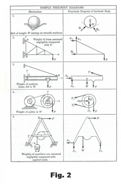
The process of drawing a free-body diagram consists of:
(1) Deciding exactly what body (or group of bodies to be regarded as a single body) is to be isolated and analyzed.
(2) Drawing an outline representing the external boundary of the body selected.
(3) Drawing in force vectors for all forces acting on the body, placing them in their correct positions. Known forces should be labeled with their magnitudes and unknown forces should be labeled with symbols.
In Fig. 2 are some examples of free-body diagrams. ( Source: J. L. Meriam. Mechanics, Part I- Statics, p.68)
Problem. A 60 lb force is required to operate the foot pedal shown in Fig. 3(a). Determine the tension in the connecting link and the force exerted by the bearing O on the lever. Consider the weight of the lever to be negligible.
Solution. We first draw a free-body diagram which is shown in 3(b). We begin by taking the moment about O, utilizing
∑MO = 0
∑MO = 9T- 60×14 = 0
so T = 93.3 lb.
We now make use of the two equations of equilibrium
∑Fx = 0, ∑Fy = 0
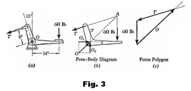
∑Fx = Ox -93.3 cos 15o = 0
so Ox = 90.1 lb.
∑Fy = Oy - 60 - 93.3 sin 15o = 0
so Oy = -84.1 lbs.
For more information and worked examples see the references below.
References
J. L. Meriam. Mechanics, Part I- Statics
Schaum. College Physics.
Faires, Chambers. Analytic Mechanics.
McLean, Nelson. Engineering Mechanics. (Schaum)
Eshbach. Handbook of Engineering Fundamentals.
The International Dictionary of Applied Mathematics. (D. Van Nostrand Co.)